Gibbs sampling is a Markov chain Monte Carlo (MCMC) algorithm used for generating samples from a complex distribution. It is a powerful tool used in various fields, such as statistics, machine learning, and computer science. In this blog post, we will discuss the concept of Gibbs sampling, its mathematical formulas, and provide a code example in Python programming language.
Gibbs sampling is a technique used to generate samples from a probability distribution that is difficult to sample from directly. Suppose we have a joint probability distribution \(P(x,y)\), where x and y are two random variables. The goal is to generate samples from the conditional probability distribution \(P(x|y)\) and \(P(y|x)\). However, if the joint distribution \(P(x,y)\) is complex, it may be difficult to sample directly from these conditional distributions.Gibbs sampling solves this problem by using a Markov chain to generate samples from the conditional distributions. At each step of the Markov chain, we sample a new value for one of the variables while holding the other variable fixed at its current value. Specifically, we alternate between sampling from the conditional distribution \(P(x|y)\) and \(P(y|x)\) until we obtain a set of samples that are approximately from the joint distribution \(P(x,y)\). The key idea behind Gibbs sampling is that by repeatedly sampling from the conditional distributions, we eventually converge to the joint distribution. This convergence is guaranteed if the Markov chain is ergodic, which means that it is irreducible and aperiodic.
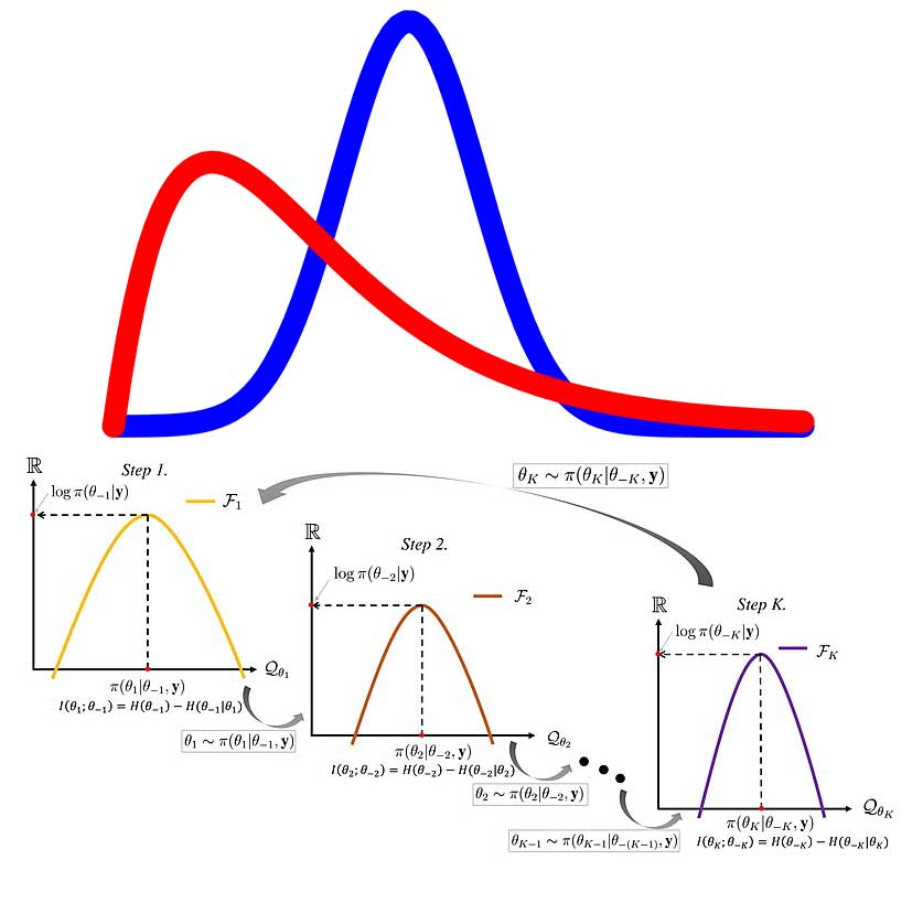
The Gibbs sampler generates samples by iterating through the following steps:
Let’s implement Gibbs sampling in Python to generate samples from a bivariate normal distribution. We will use the following joint probability distribution:
where \(\mu_x\), \(\mu_y\), \(\sigma_x\), \(\sigma_y\), and \(\rho\) are the mean and standard deviation of \(x\) and \(y\), and their correlation coefficient, respectively.
We will generate samples from the conditional distributions \(P(x|y)\) and \(P(y|x)\) using the following formulas:
Here’s the Python code to implement Gibbs sampling:
import numpy as np import matplotlib.pyplot as plt def gibbs_sampler(num_samples, mu_x, mu_y, sigma_x, sigma_y, rho): # Initialize x and y to random values x = np.random.normal(mu_x, sigma_x) y = np.random.normal(mu_y, sigma_y) # Initialize arrays to store samples samples_x = np.zeros(num_samples) samples_y = np.zeros(num_samples) # Run Gibbs sampler for i in range(num_samples): # Sample from P(x|y) x = np.random.normal(mu_x + rho * (sigma_x / sigma_y) * (y - mu_y), np.sqrt((1 - rho ** 2) * sigma_x ** 2)) # Sample from P(y|x) y = np.random.normal(mu_y + rho * (sigma_y / sigma_x) * (x - mu_x), np.sqrt((1 - rho ** 2) * sigma_y ** 2)) # Store samples samples_x[i] = x samples_y[i] = y return samples_x, samples_y # Generate samples from bivariate normal distribution using Gibbs sampling num_samples = 10000 mu_x = 0 mu_y = 0 sigma_x = 1 sigma_y = 1 rho = 0.5 samples_x, samples_y = gibbs_sampler(num_samples, mu_x, mu_y, sigma_x, sigma_y, rho) # Plot the samples plt.scatter(samples_x, samples_y, s=5) plt.title('Gibbs Sampling of Bivariate Normal Distribution') plt.xlabel('x') plt.ylabel('y') plt.show()In this code, we first define a function gibbs_sampler that takes as input the number of samples to generate ( num_samples ), the mean and standard deviation of \(x\) and \(y\) ( mu_x , mu_y , sigma_x , sigma_y ), and the correlation coefficient ( rho ). The function initializes \(x\) and y to random values and then runs the Gibbs sampler for the specified number of iterations. At each iteration, it samples a new value for \(x\) from the conditional distribution \(P(x|y)\) and a new value for \(y\) from the conditional distribution \(P(y|x)\), and stores the samples in arrays. Finally, it returns the arrays of samples for \(x\) and \(y\).
We then use this function to generate samples from a bivariate normal distribution with mean 0 and standard deviation 1 for both \(x\) and \(y\), and a correlation coefficient of 0.5 . We plot the samples using matplotlib to visualize the distribution.
If you are working on a project that involves generating samples from complex probability distributions, Gibbs sampling is an excellent choice of algorithm. It is widely used in various fields, including statistics, machine learning, and computer science, due to its simplicity and effectiveness. By iteratively generating samples from the conditional distributions of each variable given the current values of the other variables, Gibbs sampling can generate samples from joint distributions that are difficult or impossible to sample from directly. The Python code example provided above demonstrates how to implement Gibbs sampling for generating samples from a bivariate normal distribution, but the algorithm can be easily adapted to other distributions and applications.
In this blog post, we discussed the concept of Gibbs sampling, its mathematical formulas, and provided a code example in Python programming language. Gibbs sampling is a powerful tool for generating samples from complex probability distributions, and it has applications in various fields, such as statistics, machine learning, and computer science. With the code example provided, you can start using Gibbs sampling in your own projects and explore its capabilities further.