
The EU-South Korea Free Trade Agreement, which entered into force in 2015, is an example of so-called “second-generation” regional trade agreements. Using the gravity equation and drawing on a novel dataset on trade in manufacturing goods (Monteiro in World Trade Organization, Geneva, 2020), I explore the heterogeneity in the trade effects of this agreement across time (anticipation and phasing-in/delayed adjustment), country pairs, and across trading directions within pairs (exports versus imports). First, the positive trade effect after the announcement vanished one year prior to entry into force. Second, on average exports of EU countries to South Korea rise, while imports of EU countries are not significantly affected, potentially reflecting differences in ex ante trade policies. Third, additional imports caused by the agreement are larger for those EU countries where South Korea accounted for a large share of extra-EU imports already before the agreement.

Avoid common mistakes on your manuscript.
The world trading system has witnessed a proliferation of regional trade agreements (RTA) since the 1990s. While for a long time these agreements were “regional” not only in a trade-policy, but also in a geographic sense, they now span along global value chains and involve countries in different regions of the world, forming what Bhagwati has called “spaghetti bowls” (Bhagwati 1995). Moreover, they include chapters on barriers to trade other than tariffs, thus forming what is now generally referred to as “deep” agreements (WTO+ agreements).
Due to the initiative “Global Europe: Competing in the world” of 2006, the European Union (EU) is an important driver of this trend. The EU has recently signed several RTAs with countries all over the world. The EU-South Korea Free Trade Agreement is the first RTA under the “Global Europe” initative and can serve as a prominent example of these second-generation RTAs that cover tariffs, regulatory barriers, services, intellectual property rights, and bilateral investment. Footnote 1 The trade negotiations were launched in May 2007. The EU-South Korea FTA was initialled by both sides in October 2009, signed in October 2010, provisionally applied as of July 2011, and fully entered into force in December 2015 (Lakatos and Nilsson 2017).
The EU has recently signed similar agreements with Columbia and Peru (2013), Central America (2013), Canada (2017), Japan (2019), Singapore (2019), and Vietnam (2020), and has started negotiating similar agreements with Australia, New Zealand, and India. Likewise, South Korea followed a deep economic integration approach. Shortly before its agreement with the EU entered into force, South Korea entered agreements with India and the Association of Southeast Asian Nations (ASEAN) countries (both in 2010), almost at the same time an agreement with Peru (2011), and in the years thereafter agreements with the United States of America (2012), Turkey (2013), Australia (2014), Canada, China, Vietnam, and New Zealand (all in 2015), Colombia (2016), Central America (2019), and the UK (2021; substitute for the EU-South Korea FTA after the UK left the EU).
Against this background, in this paper I answer two questions: How do the trade effects of the EU-South Korea FTA differ across different phases of the agreement (pre- and post-agreement), and how do the effects differ across country pairs within the agreement as well as across directions of trade within country pairs?
According to Baier and Bergstrand (2007), an RTA – they use the term free trade agreement (FTA) – on average increases two member countries’ trade by about 100% after 10 years. This estimate is derived from a dataset that covers the period 1960-2000 (in 5-year intervals) and trade between 96 countries. Under the assumption of symmetric trade costs, they properly control for multilateral resistance terms (Anderson and van Wincoop 2003). Footnote 2 However, this study suffers from a number of deficiencies. It does not account for heteroscedasticity in the error term and zeros in international trade flows (Santos-Silva and Tenreyro 2006), nor does it allow for trade diversion from domestic trade flows (Yotov 2012), or for potential anticipation effects (Egger et al. 2022). Footnote 3 Moreover, by construction of the dataset, their estimation cannot account for the more recent RTAs such as the EU-South Korea FTA.
Using a dataset with information on both international and intra-national trade for 69 trading partners and the years 1986-2006 and estimating by Poisson Pseudo Maximum Likelihood (PPML), Baier et al. (2019) find an average trade-creating effect of 34%, accounting for 5-year lagged effects. Their analysis is restricted to RTAs that were formed in the 1980s and the 1990s. Footnote 4 Interestingly, they provide detailed evidence on differences in the effects not only across agreements, but also within agreements both across pairs and within pairs across directions of trade.
Like Zylkin (2016) for the North American Free Trade Agreement (NAFTA), I zoom into a single trade agreement, namely the EU-South Korea FTA. Footnote 5 I combine the different dimensions of heterogeneity and quantify the heterogeneity of the effects of the EU-Korea FTA across time (pre- and post-agreement), country pairs, and directions of trade (imports vs. exports) within country pairs. In order to do so, I construct a dummy variable that is 1 for each country pair involving an EU member country and South Korea for 2011 and all years thereafter and 0 otherwise. This EU-South Korea dummy variable captures the effects of all bilateral trade cost changes induced by the agreement, including changes in bilateral tariffs and in non-tariff measures (NTM), as in Baier and Bergstrand (2007). Footnote 6 Moreover, as will become clear in Sect. 2, the starting conditions in the EU and South Korea for trade liberalization within the agreement differ between the EU and South Korea as well as between different EU-countries. Thus, I will also explore directional effects (exports vs. imports). Some of the measures such as Sanitary and Phytosanitary Measures (SPS) are only applied by some of the countries to some of the trading partners within the agreement. Moreover, even NTMs that are in principle applied to all trading partners may generate asymmetric effects as the composition of bilateral trade differs. That is why I also consider country-specific and within-pair direction-specific trade effects.
All regressions include zero trade flows and are estimated using a “three-way” fixed effects Poisson Pseudo-Maximum Likelihood (“FE-PPML”) estimator with (i) exporter-and-time fixed effects and (ii) importer-and-time fixed effects to control for exporter- and importer-specific observed and unobserved characteristics such as technology, aggregate expenditure, and outward and inward multilateral resistance terms, and (iii) asymmetric pair-specific fixed effects to control for time-invariant country-pair specific characteristics. Footnote 7 These pair dummies are also thought to mitigate the potential problem of endogenous selection into RTAs (Baier and Bergstrand 2007). Following Egger et al. (2022), I use consecutive-year data in the estimation. Weidner and Zylkin (2021a, b) argue that the estimated coefficients and the standard errors obtained from three-way FE-PPML estimators are biased due to incidental parameter problems. They show that even samples with a large number of countries feature these biases. Footnote 8 Following their advice, I present bias-corrected estimates and standard errors. Footnote 9
In all regressions, I account for common globalization effects with a set of time-varying border dummy variables, separating domestic from international transactions (Bergstrand et al. 2015). I rely on a novel dataset provided by the WTO (Monteiro 2020) that contains information on international as well as on intra-national flows in manufactured goods at an annual basis for more than 180 tradings partners and for the period from 1980 to 2016, as recommended by the recent gravity literature (Yotov et al. 2016). Footnote 10 Morover, all regressions include controls for the average RTA other than the EU-South Korea FTA.
Following Baier and Bergstrand (2007), in addition to the contemporaneous effect as of 2011 (the date of provisional application), I also consider lagged trade effects. This is important when concessions are phased in over some years (Baier and Bergstrand 2007) and when the trade effects are subject to lagged adjustment. Footnote 11
Additionally, I account for anticipation effects (Egger et al. 2022). Such effects arise during the negotiation and initialling period when firms start to adjust their behavior in anticipation of the implementation of the agreement (Breinlich 2014; Moser and Rose 2014) and when uncertainty about future negative trade policy shocks is resolved. Footnote 12 Handley and Limão (2015) argue that 75% of the increase in Portugal’s exports to the EU following the 1986 enlargement can be explained by removing trade policy uncertainty. Similarly, Handley and Limão (2017) provide evidence for anticipation effects also for China’s accession to the WTO in 2001. In order to compute the cumulative effect, I sum over all coefficients.
I find that the EU-South Korea features an anticipation effect two years prior to the agreement, but this effect is eaten up by a negative trade effect one year prior to the agreement. Moreover, I find no significant trade effect in the five years after the agreement entered into force. However, this zero aggregate effect might mask heterogeneity across directions of trade. Following Civic Consulting and Ifo Institute (2018), I therefore allow the effects to differ across directions of trade. Indeed, exports from EU countries to South Korea increase on average, while the effect on EU countries’ imports from South Korea (South Korea’s exports to EU countries) is insignificant.
I find huge heterogeneity in the trade effects across country pairs. The cumulative trade effects are significantly positive for trade between South Korea and Croatia, Czech Republic, Greece, Lithuania, Poland, Romania, Slovakia, and Slovenia and significantly negative for trade between South Korea and Bulgaria and Finland. There is also heterogeneity within pairs across directions.
The literature discusses several potential explanations for asymmetries in the effects of trade liberalization across country pairs. Kehoe and Ruhl (2013) and Baier et al. (2019) report evidence in favor of the hypothesis that country pairs trading a smaller range of product varieties before the trade negotiations start have a higher potential for trade growth thereafter. Zylkin (2016) argues that the heterogeneity in trade effects on different members can be expected to be explained by differences in ex ante trade barriers, but he finds the trade effects of the North American Free Trade Agreement (NAFTA) to “disagree strongly with expectations based on pre-NAFTA tariffs.” (p. 1). Larch et al. (2021) report that the trade effects of the EU-Turkey Customs Union are negatively correlated to inital bilateral trade barriers, as measured by the asymmetric pair fixed effect. In the context of Canada’s trade agreements, Anderson et al. (2017) stress that differential trade effects on member countries of an RTA “are not a reflection of comparative advantage, since comparative advantage forces and their changes over time are already controlled for [. ] by the exporter-time and the importer-time fxed effects” (p. 35). They propose unobserved trade policy variables as well as outsourcing patterns as potential explanations.
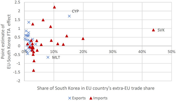
In this paper, I relate the directional trade effects on EU member countries to the shares of the South Korea in extra-EU exports and imports, respectively, but I do not take a stance on what type of relationship between initial trade levels and trade growth induced by the agreement to expect. I find the directional trade effects to be positively correlated to the share of South Korea in the EU country’s extra-EU imports in the year 2010. Footnote 13
I am not the first to look into the trade effects of the EU-South Korea FTA. In a report to the European Commission, Civic Consulting and the Ifo Institute (2018) discuss the concessions and the effects of the EU-Korea FTA in great detail. They find a positive effect on both EU exports to and EU imports from Korea. The latter is estimated to be smaller than the former. I find a similar pattern, the difference being that in my estimations the effect on imports of EU countries is not statistically significant. The empirical analysis in Civic Consulting and Ifo Institute (2018) is based on information from the World Input Output Database (WIOD) (Timmer et al. 2015). In the regressions, the authors pool across all available sectors, which also includes agricultural, mining, and services sectors. The authors also provide estimates of sectoral directional effects. The effect on EU exports to South Korea is significantly positive for most of the sectors, while the effects on EU imports from South Korea are more mixed. In particular, there is no significant effect on imports of Computer, Electronic and Optical Equipment and Electrical Equipment (see their Table 91), which are quantitatively important sectors (see below).
Grübler and Reiter (2021) find that the EU-South Korea FTA increases bilateral trade on average by 9.42%, which is smaller than my estimate. In their regressions, they do neither account for anticipation nor for delayed effects. They also disentangle the effects of tariffs and non-tariff measures (NTMs). In the regressions where they separately control for tariffs, the EU-South Korea FTA dummy does not show up significantly. This suggests that NTMs have on average no additional role in explaining trade flows, once tariffs are controlled for. I stick to the ‘umbrella’ approach with a single dummy that picks up changes in tariffs and NTMs, but additionally explore anticipation and delayed effects as well as directional effects.
Juust et al. (2020) use a sample of 36 countries for the period 2005-2015. Thus, the number of trading partners is very small. Moreover, the dataset only covers two years prior to the launch of the trade negotiations. They also find differential effects on EU exports to and imports from Korea. In their regressions, they focus on the transition periods 2011-2013 and 2011-2015. I consider the period from 1980-2016 (and RTAs until 2021) and estimate directional effects also within country pairs.
Using product level data, Lakatos and Nilsson (2017) show that, compared to the period before negotiations began, the EU-South Korea FTA had a positive impact on trade during the start of negotiations (June 2007) and after the initialling of the agreement (Sept 2009). While their dataset contains detailed (8-digit) product-level information on trade between EU countries and South Korea, I consider trade at the aggregate (manufacturing) level, but include other countries as well in order to be able to properly control for country-specific effects and other free trade agreements. Moreover, I also account for delayed effects.
The paper is also related to Larch et al. (2021) who explore the average and the heterogeneous effects of the EU-Turkey Customs Union. They use a similar approach, allow additionally for heterogeneity across sectors, but use a shorter dataset (1988-2006) and do not apply bias corrections.
The remainder of the paper is organized as follows. In Sect. 2, I give an overview of the trade environment before and after the EU-South Korea FTA. In Sects. 3 and 4, respectively, the structural gravity framework and the data are presented. Section 5 contains the econometric specifications and results. The final section discusses explanations for the observed heterogeneity in the trade effects.
In this section, I take a general perspective and give a first impression of EU-South Korea trade before and after the agreement to get a sense of the magnitudes. In Sect. 3, I aim at causality and use the gravity equation to establish a norm against which to measure trade effects, controlling for all factors other than the trade agreement that affect trade cross-country and over time.
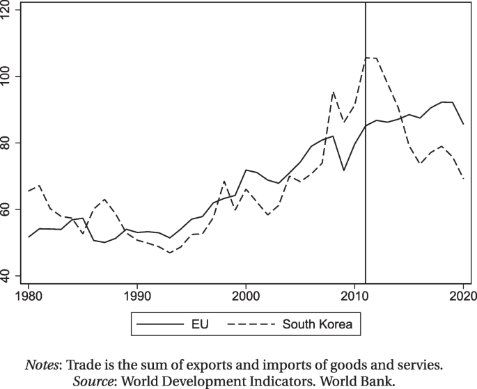
In order to illustrate how the EU and South Korea are integrated into the world economy, Fig. 1 displays their trade-to-GDP ratios for the year 1980-2020. Footnote 14 While these ratios moved in tandem more or less until 2007, South Korea’s ratio exceed that of the EU in 2008, reached its peak in 2011 (around 106%), but then fell to around 74% in 2016. The period of this drop coincides with the five years after the implementation of the EU-South Korea FTA. In the EU, the ratio increased only modestly, but steadily between 2008 (82%) and 2019 (92%), with a drop in 2009 due to the crisis. In the regression analysis below, the movements of the countries’ trade orientations will be captured by (role-specific country-and-time) fixed effects.
Table 1 lists the top trading partners of the EU and of South Korea for the years 2010 (one year before the agreement entered into force) and 2016 (five years after the agreement entered into force). In line with the regression analysis below, the numbers refer to trade in manufactured goods in current prices. With a volume of 34,841 billions USD, South Korea was the tenth largest destination for EU exports in 2010 (2.2% of total extra-EU exports) and the nineth largest export destination in 2016 (2.6%). South Korea was the sixth largest source country of EU imports in 2010 (4.2%) and the seventh largest source country in 2016 (3.6%). Thus, South Korea is in the group of the top ten trading partners of the EU, but only at the lower end when it comes to export destinations. Moreover, the share of imports from South Korea in total EU imports slightly declined between 2010 and 2016.
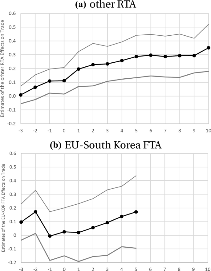
The EU-South Korea FTA effects show a different pattern. There are statistically significantly positive effects two year prior to the agreement, but these effects have vanished one year prior to the agreement. Starting from one year after the agreement entered into force, the effect steadily rises, but after a 5-year period, its magnitude is only comparable to the one other RTAs have reached after two years. Moreover, the effect is not statistically significant.
Finally, I present results from a regression where I use a somewhat coarser time structure. More precisely, I only consider the 3-year lead, the 5-year lag, and for other RTAs additionally the 10-year lag. Columns (4) and (5) of Table 3 show the result. In Column (4), I use the standard dataset. The 3-year leads are not statistically significant. The contemporaneous effect of other RTAs is large and highly significant, while the one of the EU-South Korea FTA is not. Both 5-year lags are positive and statistically significant. The cumulative effects obtained from this specification are comparable to the ones obtained from a specification with annual leads and lags, compare columns (2) and (3). In Column (5), I repeat the exercise on the smaller dataset that only contains 76 countries. This leaves the estimates of the trade effects of other RTAs by are large unchanged. The estimates of the trade effects of the EU-South Korea FTA are somewhat smaller.
The estimates obtained in the previous subsection represent the effect of the EU-South Korea FTA on bilateral trade between EU member countries and South Korea. Almost any theory of specialization suggests the effects to be different for imports and export. I therefore now allow the effect to differ across directions of trade d, where d can be either exports or imports. Footnote 29 More specifically, I run the following regressions
$$\begin
Along with the contemporaneous effect, I consider the 3-year lead and the 5-year lag. For other RTAs, I additionally include the 10-year lag.
Table 4 displays the results. The effects of other RTAs are not affected by allowing for heterogeneity across directions of the EU-South Korea FTA, compare Table 4 to column (4) of Table 3. There are, however, differences in the effect of the EU-South Korea FTA across directions. The cumulative effect of the EU-South Korea FTA on exports of EU countries to South Korea is 0.329 (with a standard error of 0.155), which implies an increase in bilateral trade by \(39\%\) . Footnote 30 This effect is smaller than the one reported by Civic Consulting and Ifo Institute (2018), who report a trade effect of \(54\%\) on exports of EU countries to South Korea. Recall, however, that while the present analysis takes two more years of adjustment into account, it is limited to manufactured goods. The cumulative effect of the EU-South Korea FTA that materializes after five years is slightly larger, however, than the effect that other RTAs reach after ten years, and substantially larger than the effect that other RTAs reach after five years.
Second, country pairs may also differ in the range of products they trade with each other. Kehoe and Ruhl (2013) argue that country pairs trading a smaller range of product varieties before the trade negotiations start have a higher potential for trade growth thereafter. In the present paper, I do not explore their “least-traded goods hypothesis”.
Third, through the lens of the model, the estimated coefficients compound the semi-elasticity of trade costs in the RTA with the elasticity of bilateral trade in bilateral trade costs. In an Armington (1969) or a Krugman (1980) setting, the latter is governed by the elasticity of substitution between varieties. Footnote 39 These elasticities differ across products (Rauch 1999). Products featuring a low elasticity of substitution respond less to a given trade cost shock compared to products characterized by a large elasticity of substitution. Hence, when the product composition of trade flows differs across directions within pairs, the trade effects will differ as well.
In this paper, I document substantial heterogeneity in the partial effects of the EU-South Korea FTA across time, country pairs, and directions within country pairs on bilateral trade in manufactured goods. In doing so, I contribute to the recent literature that stresses heterogeneity in the effects of trade policy changes. I find the phasing-in period of five years to be too short to find a significant average trade effect of the EU-South Korea FTA. Moreover, I fail to find a significant effect on EU imports of manufactured goods from South Korea. This implies that the positive effect on imports found by Civic Consulting and Ifo Institute (2018) must be driven by sectors other than manufacturing. Differences in the effects on EU exports and EU imports, however, are likely to reflect differences in ex ante trade barriers. Regarding country-specific estimates, I find significiant effects mainly for countries that have joined the EU relatively recently. Thus, the coefficients may reflect adjustments to EU membership or differences in the composition of trade with South Korea between new and old EU members. I find a positive correlation between directional trade effects and the inital share of South Korea in extra-EU-imports.
For a better understanding of the effect, it would be interesting to explore the margins through which the EU-South Korea FTA affects bilateral trade volumes. Using French customs data, Chowdhry and Felbermayr (2021) find that firms that are larger before the EU-South Korea FTA benefit more in terms of sales from the FTA than firms at the lower end of the size distribution.
Some of the estimated cumulative partial trade effects seem to be negative, which is not a new result. Baier et al. (2019) find a substantial share of agreement-by-pair and agreement-by-direction effects of the EU accession and other agreements to be negative; see their Table 2 and their Fig. 2. Footnote 40
The structural gravity system described in Sect. 3 can be derived under different sets of assumptions (Yotov et al. 2016). There are trade models, however, that do not predict a multiplicative form of the gravity equation. Footnote 41 Examples are gravity equations derived from linear demand systems (Ottaviano et al. 2002; Spearot 2013) or translog expenditure functions (Feenstra 2003; Novy 2013; and Chen and Novy 2021). Also in models with endogenous marketing costs, the effect of trade liberalization on small firms differs from the one on large firms, which makes the response of aggregate trade dependent on the composition of firms (Arkolakis 2010). Irarrazabal et al. (2015) explore the gravity equation – at the firm-level – in the presence of additive trade costs. Moreover, Adão et al. (2020) allow for a flexible parametrization of the productivity distribution in a monopolistic competition model with firm heterogeneity. There are also truely trade dynamic models (e.g., Alessandria et al. 2021). In all these models, trade elasticities are not constant. More importantly, they command a different specification of the gravity equation.
I leave a more sophisticated explanation for the heterogeneity of the trade effects and the use of other specifications of the gravity equation to future research. Moreover, it would be interesting to bring in other sectors like the service sectors again.
The World Trade Organization (WTO) classifies the following types of RTAs, defined under the General Agreement on Tariffs and Trade (GATT) and the General Agreement on Trade in Services (GATS): Customs Union (CU), Economic Integration Agreement (EIA), Free Trade Agreement (FTA), and Partial Scope Agreement (PSA). RTAs can be combinations of different types. In fact, the EU South-Korea FTA is classified as “FTA & EIA”.
In the regressions, they include country-and-time fixed effects rather than exporter-and-time and importer-and-time fixed effects. This is adequate only under the assumption of symmetric trade costs and the absence of trade deficits, because only then the outward and the inward multilateral resistance terms coincide, such that country-and-time effects suffice to control for both, outward and inward multilateral restistance.
The presence of domestic trade flows is also important to be able to identify trade diversion effects of RTAs (Dai et al. 2014).
As they include a 5-year lag, they can include RTAs that entered into force until 2001.Baier et al. (2019) zoom into all RTAs in their dataset. Egger et al. (2022) use the same dataset as Baier et al. (2019), but mainly focus on the different phases that characterize the impact of the average RTA on bilateral trade and also explore the phases of the Canada-Chile Free Trade Agreement (CCFTA) and the Canada-Israel Free Trade Agreement (CIFTA), both launched in 1997.
Chowdhry and Felbermayr (2021) call this an ‘umbrella’ approach.I use the command ppmlhdfe provided by Correira et al. (2019) and described in more detail in Correira et al. (2020).
In their Table 5, Weidner and Zylkin (2021a) show i.a. the biases for the data used in Larch et al. (2019a), whose dataset contains even more countries and more time periods than the one in the present dataset.
I use the command ppml_fe_bias proved by Weider and Zylkin (2021b). However, Stata runs against the memory constraints of the server and exits with an error in the pair-specific regressions. For these regressions, I use a smaller dataset; see below.
The dataset is also used by Larch et al. (2019b). There are alternative datasets that also feature intra-national trade. The dataset used by Baier et al. (2019) only covers the years 1986-2006 and therefore is not suited to study the trade effects of the EU-South Korea FTA. The second release of the World Input Output Database (WIOD, Timmer et al. 2015) covers the years 2000-2014, which only leaves room for a shorter phasing-in period. Moreover, Borchert et al. (2021) advise against using the WIOD data for estimation purposes because it “relies on economic models to estimate missing data” (p. 163). The International Trade and Production Database (Borchert et al. 2021) contains information at a more detailed industry level and additionally includes industries from agriculture, mining and energy, and services. However, as the dataset is unbalanced (some countries do not appear in some years and/or industries), one cannot aggregate up to these “broad sectors”. One could estimate industry-by-industry, but in the present context, this procedure would result in an unmanagable number of estimated coefficients. An alternative would be to pool across industries, but the biases that may arise in “four-way” gravity models have not been fully characterized yet (Weidner and Zylkin 2021a, p. 13).
Think of a machine that is ordered today but delivered only in the next year. This effect is conceptionally different from a dynamic adjustment that arises in models where foreign market entry costs are sunk (Das et al. 2007; Alessandria and Choi 2014) or the structure of export costs involves risk (Alessandria et al. 2021), which would command a dynamic specification of the gravity equation.
A new situation already arises with the beginning of the negotiations. As they continue, the uncertainty is gradually reduced.
For exports, the picture is less clear. Ignoring Cyprus, the correlation between the trade effect and the share of South Korea in the EU country’s extra-EU exports is negative, but with Cyprus, it is also positive.
In this figure, trade is the sum of exports and imports of goods and services.The list of South Korea’s top 10 export destinations for manufactured goods in 2016 includes the Marshall Islands (1.6%). Note that also Malaysia (MYS) and Australia (AUS) reveive a share of 1.6% of exports from South Korea. Moreover, the export shares that go Philippines (PHL) and India (IDN) are 1.5% and 1.4%. In 2010, Malaysia received 1.1% of exports from South Korea.
Aggregate expenditure can also be expressed in terms of nominal income as \(E_
The number of leads s and lags k taken into account, however, is restricted to be the same for all RTAs.
Note that \(X_
The data do neither cover trade in agricultural products, fuels, and minining products nor in services.
The alpha-3 country ISO code of the conglomerate “Belgium-Luxembourg” is BLX. For country and year coverage, see Monteiro (2020).In the regressions, I include lagged information on RTA membership. For example, in regressions with a 10-year lag, bilateral trade in the year t (say, 1980), is related to the existence of an RTA in the year \(t-10\) (say, 1970).
For the year 2021, I only include RTAs that entered into force and appeared in the Database by July 7, 2021; see Table 8 in the Appendix for a list of RTAs that entered into force in 2020 and 2021. Most of the 42 agreements that entered into force in 2021 are agreements that involve the UK and substitute for agreements the UK formerly had under the umbrella of the EU, which has no effect on the coding of the RTA dummy.
Croatia joined the EU only in 2013 (and immediately entered the EU-South Korea FTA), so in regressions where I include country pairs separately, the number of lags for Crotia is restricted to 3.
In a regression with a 5-year RTA lead, bilateral trade in the year t (say, 2016) is related to the existence of an RTA in the year \(t+5\) (say, 2021).
The 7 additional countries are the Croatia (HRV), the Czech Republic (CZE), Estonia (EST), Latvia (LVA), Lithuania (LTU), Slovakia (SVK), and Slovenia (SVN).
For the sake of the focus on the EU-South Korea FTA, I ignore heterogeneity in the group of other RTAs.
Baier and Bergstrand (2007) and Egger et al. (2022) find negative 5-year leads for RTAs.Baier et al. (2019) who explore heterogeneous RTA effects warn that “[w]hile Baier and Bergstrand (2007) has emerged as the standard method for consistently estimating the average treatment effect of FTAs, the same cannot be said when we pull apart our average “ \(\beta\) ” to obtain increasingly more finely-grained coefficients, which we should regard as being estimated with at least some unobserved error” (p. 210). In the present analysis, I only zoom into a single RTA, as in Egger et al. (2022) and Larch et al. (2021).
With \(\sigma =5\) , this implies a reduction in bilateral trade frictions by approx. \(6.4\%\) .As Croatia (HRV) joined the EU and hence the EU-South Korea Agreement only in 2013, I include lag 3 rather than lag 5.
Recall that Belgium and Luxembourg are merged to Belgium-Luxembourg in the trade data, such that in total there are 27 country pairs.
Baier et al. (2019) also find negative pair-specific EU accession effects for 24 country pairs. The only exception is Greece. For Bulgaria, a significantly negative effect arises. Table 9 in the Appendix display the results for the full sample, but without bias correction.The significantly negative cumulative effects arise for Bulgaria (both trade directions), for exports of Malta, and imports of Denmark, Finland, and Ireland. Baier et al. (2019) report negative EU accession effects for some directed pairs. Larch et al. (2021) find negative effects on exports from Cyprus and Malta to Turkey
The exceptions are Finland and Greece.Note that Baier et al. (2019) and Larch et al. (2021) relate the estimated directed trade effects to the estimated pair fixed effects, while I use an observed measure of trade openness.
In the Melitz (2003)-cum-Pareto model, this is the shape parameter of the Pareto distribution.They also warn that the specific estimates are likely to “reflect omitted factors that may enter [the] specifications [. ] via the error term” (p. 215).
Head and Mayer (2014) conclude that “the main reason to insist on the multiplicative form in the definition of gravity is historical usage. It is therefore possible that future work would abandon the multiplicative form and redefine gravity to allow other functional forms.” (p. 138).
I am grateful to Wilhelm Kohler and Julia Spornberger for thoughtful dicussions and comments. I am also grateful for comments from participants of the Hagen Workshop on Global Economic Studies in May 2021 and from two anonymous referees. I also thank Tom Zylkin for sharing the bias-correction command ppml_fe_bias_savev that saves the variance-covariance matrix. All remaining errors are mine.
Open Access funding enabled and organized by Projekt DEAL.
